I accidentally implemented the fastest pairwise cosine similarity function

While searching for a way to efficiently compute pairwise cosine similarity between vectors, I created a simple and efficient implementation using PyTorch. The function runs blazingly fast. It is faster than the popular cosine_similarity function from sklearn and the naive loop-based implementations.

1
2
3
4
5
6
7
8
9
10
11
12

def pairwise_cosine_similarity(tensor: torch.Tensor) -> torch.Tensor:
    """
    Args:
        tensor: A tensor of shape (N, D) where N is the number of vectors and D is the dimensionality of the vectors.
    Returns:
        A tensor of shape (N, N) containing the cosine similarity between all pairs of vectors.
    """

    tmm = torch.mm(tensor, tensor.T)
    denom = torch.sqrt(tmm.diagonal()).unsqueeze(0)
    denom_mat = torch.mm(denom.T, denom)
    return torch.nan_to_num(tmm / denom_mat)

About cosine similarity

Cosine similarity is a intuitive metric to measure similarity between two vectors. It is widely used in vision, recommendation systems, search engines, and natural language processing. The cosine similarity between two vectors is defined as the cosine of the angle between them, ranging from -1 to 1, where 1 means the vectors are identical, -1 means they are opposite, and 0 means they are orthogonal.

Edit (March 2024): Be cautious about using cosine similarity when working with embeddings. Please check out Is Cosine-Similarity of Embeddings Really About
Similarity?

The use case

We usually want to compute the cosine similarity between all pairs of vectors. This enables do things like searching for similar vectors (similar images), analyzing the structure of the vector space (clustering images). However, with a large matrix, computing the cosine similarity can be computationally expensive.

We often find ourselves having a matrix of shape $(N, D)$ where $N$ is the number of vectors and $D$ is the dimensionality of the vectors. $D$ is also called the embedding size or dimension, which is typically a power of 2, e.g. 64, 512, 1024, 4096, etc.

The method

The method is based on the following formula:

$$\text{sim}(v_i, v_j) = \frac{v_i \cdot v_j}{\lVert v_i \rVert \lVert v_j \rVert}$$

Let’s explain what the code does:

1
2
3
4

tmm = torch.mm(tensor, tensor.T)
denom = torch.sqrt(tmm.diagonal()).unsqueeze(0)
denom_mat = torch.mm(denom.T, denom)
return torch.nan_to_num(tmm / denom_mat)

1. Numerator matrix: Dot product via matrix multiplication tmm = torch.mm(tensor, tensor.T)

   This line computes the matrix multiplication of the input tensor with its transpose tensor.T. The result is a tensor tmm of shape $(N, N)$ where each element $(i, j)$ represents the dot product of vectors $i$ and $j$.

2. Denominator values: Norm of each vector denom = torch.sqrt(tmm.diagonal()).unsqueeze(0)

   The diagonal of the tensor tmm contains the dot products of each vector with itself. Taking the square root of these values gives the magnitude (or norm) of each vector. The unsqueeze(0) function is used to add an extra dimension to the tensor, changing its shape from $(N,)$ to $(1, N)$.

3. Denominator matrix denom_mat = torch.mm(denom.T, denom)

   This line computes the outer product of the vector denom with itself, resulting in a matrix denom_mat of shape $(N, N)$. Each element $(i, j)$ of this matrix is the product of the magnitudes of vectors $i$ and $j$.

4. NaN removal return torch.nan_to_num(tmm / denom_mat)

   Finally, the cosine similarity between each pair of vectors is calculated by dividing the dot product matrix tmm by the matrix denom_mat. The division is element-wise, so each element $(i, j)$ of the resulting matrix represents the cosine similarity between vectors $i$ and $j$. torch.nan_to_num is used to replace any NaN values that might occur during the division with zeros.

The output is a symmetric matrix where the diagonal elements are all 1 (since the cosine similarity of a vector with itself is always 1), and the off-diagonal elements represent the cosine similarity between different pairs of vectors!

Benchmarking

Versus naive loops, our approach completely outperforms them by several orders of magnitude. Versus sklearn.metrics.pairwise.cosine_similarity, our implementation is 10x faster, and versus a numpy implementation using the exact same logic, our PyTorch code is about 2-3x faster.

Results

1
2
3
4
5
6
7
8
9
10
11

Result within 1e-8 of scipy loop: True
Result within 1e-8 of numpy loop: True
Result within 1e-8 of torch loop: True
Result within 1e-8 of sklearn: True
Result within 1e-8 of numpy matrix: True
scipy loop:   142362.0 us
numpy loop:   112752.9 us
torch loop:   83144.2 us
sklearn:      401.8 us
numpy matrix: 136.2 us
✨ ours:      48.6 us

Benchmark code

Here is the benchmark code if anybody wishes to reproduce it:

1
2
3
4
5
6
7
8
9
10
11
12
13
14
15
16
17
18
19
20
21
22
23
24
25
26
27
28
29
30
31
32
33
34
35
36
37
38
39
40
41
42
43
44
45
46
47
48
49
50
51
52
53
54
55
56
57
58
59
60
61
62
63
64
65
66
67
68
69
70
71
72
73
74
75
76
77
78
79
80
81
82
83
84
85
86
87
88
89
90
91
92
93
94
95
96
97
98
99
100
101
102
103
104
105
106
107
108
109
110
111
112
113
114

import torch
import numpy as np
import scipy
from sklearn.metrics.pairwise import cosine_similarity


def torch_loop_cosine_similarity(tensor, output):
    for i in range(len(tensor)):
        for j in range(len(tensor)):
            output[i, j] = torch.cosine_similarity(
                tensor[i].unsqueeze(0), tensor[j].unsqueeze(0)
            )
    return output


def scipy_loop_cosine_similarity(tensor, output):
    for i in range(len(tensor)):
        for j in range(len(tensor)):
            output[i, j] = scipy.spatial.distance.cosine(tensor[i], tensor[j])
    return output


def numpy_loop_cosine_similarity(tensor, output):
    for i in range(len(tensor)):
        for j in range(len(tensor)):
            output[i, j] = float(
                np.dot(tensor[i], tensor[j])
                / (np.linalg.norm(tensor[i]) * np.linalg.norm(tensor[j]))
            )
    return output


def numpy_matrix_cosine_similarity(tensor):
    tmm = np.matmul(tensor, tensor.T)
    denom = np.sqrt(tmm.diagonal()).unsqueeze(0)
    denom_mat = np.matmul(denom.T, denom)
    return np.nan_to_num(tmm / denom_mat)


def torch_matrix_cosine_similarity(tensor):
    tmm = torch.mm(tensor, tensor.T)
    denom = torch.sqrt(tmm.diagonal()).unsqueeze(0)
    denom_mat = torch.mm(denom.T, denom)
    return torch.nan_to_num(tmm / denom_mat)


if __name__ == "__main__":

    # Create a random data tensor of shape (N=50, D=64)
    data = torch.rand((50, 64))

    # Create the output tensor
    zeros = torch.zeros((data.shape[0], data.shape[0]))

    # Compare across different implementations
    sklearn = torch.Tensor(cosine_similarity(data, data))
    npy_matrix = torch.Tensor(numpy_matrix_cosine_similarity(data))
    npy_loop = numpy_loop_cosine_similarity(data, zeros)
    spy_loop = scipy_loop_cosine_similarity(data, zeros)
    torch_loop = torch_loop_cosine_similarity(data, zeros)
    ours = torch_matrix_cosine_similarity(data)

    print(f"Result within 1e-8 of scipy loop: {bool(torch.allclose(ours, spy_loop))}")
    print(f"Result within 1e-8 of numpy loop: {bool(torch.allclose(ours, npy_loop))}")
    print(f"Result within 1e-8 of torch loop: {bool(torch.allclose(ours, torch_loop))}")
    print(f"Result within 1e-8 of sklearn: {bool(torch.allclose(ours, sklearn))}")
    print(
        f"Result within 1e-8 of numpy matrix: {bool(torch.allclose(ours, npy_matrix))}"
    )

    import timeit

    t0 = timeit.Timer(
        stmt="torch_loop_cosine_similarity(data, output)",
        setup="from __main__ import torch_loop_cosine_similarity; import torch; output = torch.zeros((data.shape[0], data.shape[0]));",
        globals={"data": data},
    )

    t1 = timeit.Timer(
        stmt="cosine_similarity(data, data)",
        setup="from __main__ import cosine_similarity",
        globals={"data": data},
    )

    t2 = timeit.Timer(
        stmt="scipy_loop_cosine_similarity(data, output)",
        setup="from __main__ import scipy_loop_cosine_similarity; import torch; output = torch.zeros((data.shape[0], data.shape[0]));",
        globals={"data": data},
    )

    t5 = timeit.Timer(
        stmt="numpy_loop_cosine_similarity(data, output)",
        setup="from __main__ import numpy_loop_cosine_similarity; import torch; output = torch.zeros((data.shape[0], data.shape[0]));",
        globals={"data": data},
    )

    t3 = timeit.Timer(
        stmt="numpy_matrix_cosine_similarity(data)",
        setup="from __main__ import numpy_matrix_cosine_similarity",
        globals={"data": data},
    )

    t4 = timeit.Timer(
        stmt="torch_matrix_cosine_similarity(data)",
        setup="from __main__ import torch_matrix_cosine_similarity",
        globals={"data": data},
    )

    print(f"scipy loop:   {t2.timeit(100) / 100 * 1e6:>5.1f} us")
    print(f"numpy loop:   {t5.timeit(100) / 100 * 1e6:>5.1f} us")
    print(f"torch loop:   {t0.timeit(100) / 100 * 1e6:>5.1f} us")
    print(f"sklearn:      {t1.timeit(100) / 100 * 1e6:>5.1f} us")
    print(f"numpy matrix: {t3.timeit(100) / 100 * 1e6:>5.1f} us")
    print(f"✨ ours:     {t4.timeit(10) / 100 * 1e6:>5.1f} us")

Contextual placement using pre-trained vision models

Early on in Bifrost’s journey, we took the simplest approach to create object detection scenarios: composite objects randomly on backgrounds. However, as contextual placement became necessary, the approach didn’t scale.

Why contexual? We need to create specialized samples to reinforce distributions and correlations in synthetic datasets. Object detectors trained on synthetic data, for instance, can fail on objects in rare or unrepresented contexts (referring to the environmental pixels surrounding the object), like aircrafts in grassy fields, or large boats in shipyards instead of on water.

We thus built a smarter, but simple, method of determining suitable placement areas in large images, which we endearingly named Mise en Place.

Embedding image areas into vectors

The early layers in trained convolutional neural networks are powerful feature extractors, even on smaller inputs^[1]. We can exploit these layers to project small areas of the image into a feature embedding space, in which the embedding vectors have some notion of vector similarity.

Here’s how it works. We first split the original tile into a grid, feeding each individual cell into the initial layers of a pre-trained network (which collectively act as an encoder) and obtaining an embedding vector for that cell:

This vector acts as a latent representation of the content of the input cell.

We then compute the cosine similarity between each cell’s embedding vector $(v_i)$, and every other vector $(v_j)$, for every $(j \in S \setminus i)$, $$\text{sim}(v_i, v_j) = \frac{v_i \cdot v_j}{\lVert v_i \rVert \lVert v_j \rVert}$$

Why not just compare the images directly?

Evidently, similar cells produce vectors similar to each other. Now, one may wonder, why bother transforming the image cell into a vector? Why not simply calculate the similarity (or difference) of the input cell directly? Here’s the problem.

Say we’re contrasting two cells (X) and (Y) by taking the sum of the absolute differences between corresponding pixel values:

$$\text{dist}(X, Y) = \sum_{i,j} \left\lvert,X_{i,j} - Y_{i,j},\right\rvert$$

For the pairs below, the top pair has a total difference of (951103), and the bottom (490118). What’s happening here?

Let’s look at the top row. The two cells seem visually similar, but the position of the diagonal feature doesn’t line up perfectly. This causes the absolute difference between the two images to be large, showin up as white areas in the difference map.

On the other hand, the bottom pair of cells don’t look similar at all, and ar likely from different areas of the original image. But their difference remains low, since pixel value coincidentally match at the same locations, resulting in a lower difference score.

The usefulness of the neural network her is in its translationally-invariant representation of the features in the image, creating embedding vectors that encode the content of each cell, rather than their literal values.

Selecting matching vectors

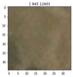
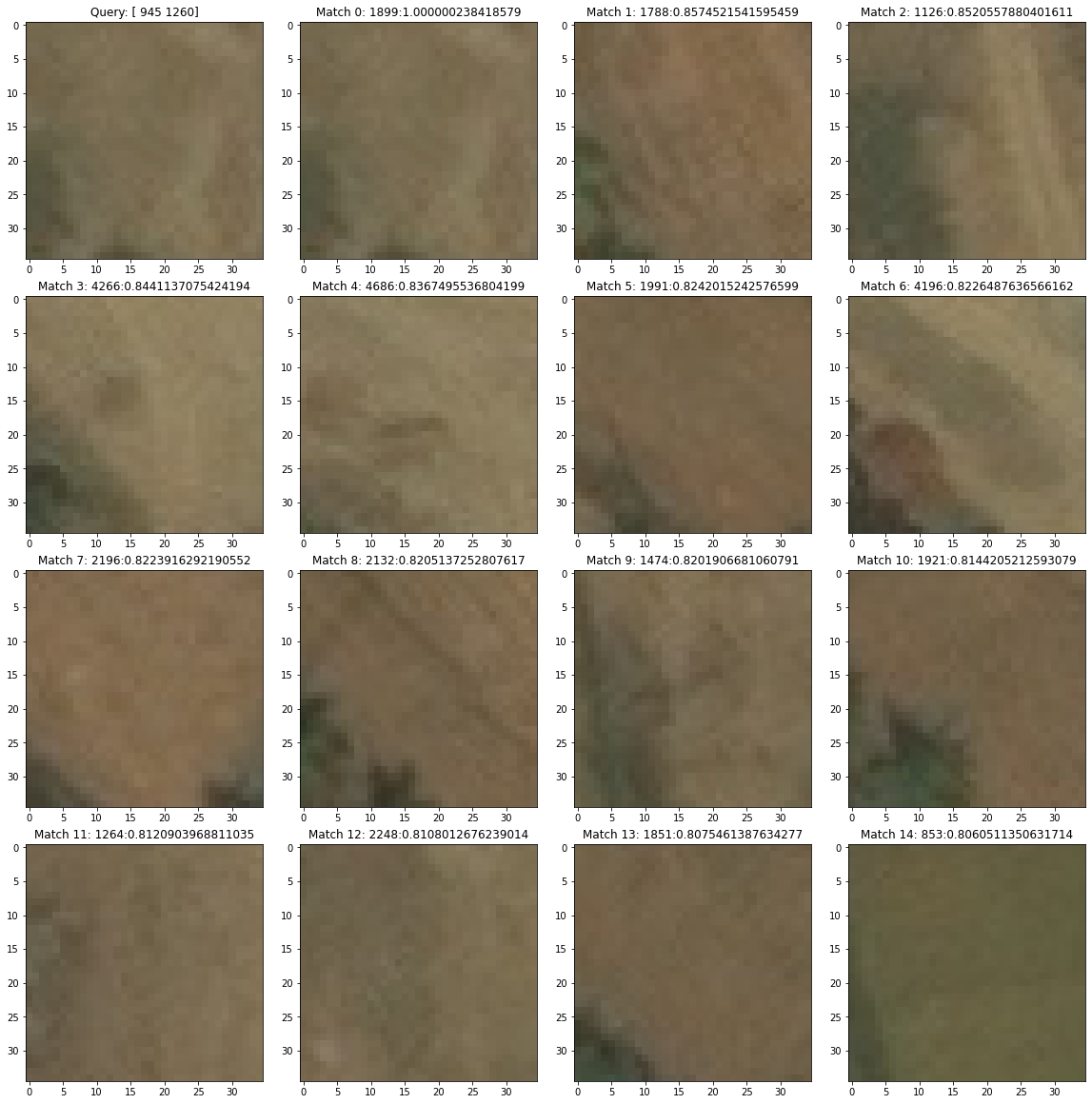
Now that we’ve scored our cells, we’ll want to query a single cell, and search for all the similar cells in the image. For instance, we’ve got this snazzy looking cell of… dirt over here.

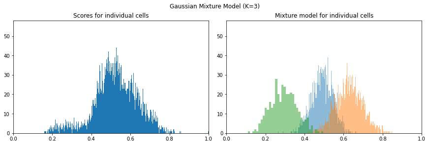
Since we have this query’s similarity scores for every cell, we can rank the cells, filtering those most similar to it. The naïve approach is to choose the top-(k) similar cells, but the manual task of determining the optimal number of cells remains. An alternative is to let the image speak for itself: we’ll break down the distribution of scores into a Gaussian mixture model^[2] and select cells belonging to the highest-scoring cluster.

Doing science

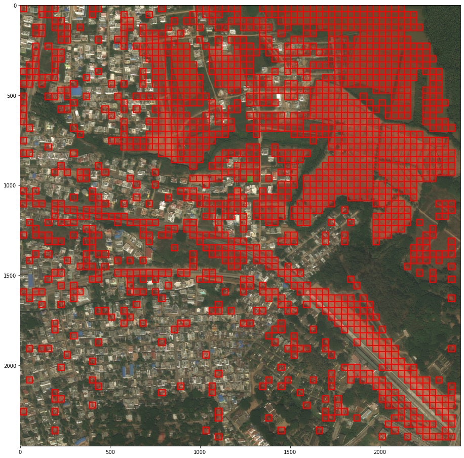
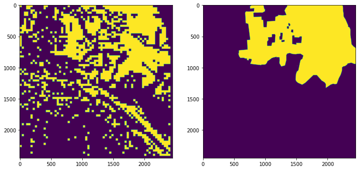
We might have managed to produce a visually consistent result, but we’ll also need to design a performance metric, which lets us perform science: tweak parameters and measure how things change. From the final group of similar cells, we can recover a coarse segmentation mask, compared to the original land-cover segmentation mask on the right. Though we’ve managed to match a significant proportion of the cover, we’ve also let too much through.

To quantify our closeness to the original segmentation mask, we’ll employ the Jaccard index^[3], or intersection-over-union (IoU):

$$J(y, \hat{y}) = \frac{\lvert y \cap \hat{y} \rvert}{\lvert y \cup \hat{y} \rvert} = 0.447$$

That’s great! Now we’re able to tweak some design choices and observe how close our results are to the ground-truth segmentation.

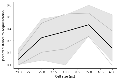
For instance, we can vary the cell size, and track its effect on the Jaccard index. For each cell size, we’d take the average IoU over 5 runs, using a random query cell each time. This hints that the optimal cell size for this particular image is around 35px – if we’re restricting ourselves to a fixed cell size, we can run this experiment over many images and try and determine the best average case.

Conclusion

This was a useful early approach to distribute objects on underrepresented areas. Though this method retains and leverages the raw power of a trained neural network, it’s fast and quick to develop, since no training is involved!

References

1. 1.Sergey Zagoruyko, & Nikos Komodakis (2015). Learning to Compare Image Patches via Convolutional Neural Networks. arXiv preprint arXiv: Arxiv-1504.03641.
2. 2.Duda, R., & Hart, P. (1973). Pattern classification and scene analysis. (Vol. 3) Wiley New York.
3. 3.Jaccard, P. (1912). THE DISTRIBUTION OF THE FLORA IN THE ALPINE ZONE. New Phytologist, 11(2), 37-50.